
Two identical centrifugal pumps in parallel usually increase flow, but the new flow is found where their combined pump curve meets the system curve. Doubling the flow of one pump at a chosen head constructs a point on the combined curve. It does not, by itself, predict what the greenhouse will receive.
This distinction matters when an expansion quote promises twice the irrigation capacity simply because a second pump has been added. Ask to see how the quoted duty follows from both curves before committing the additional crop area.
Build the parallel curve before reading the operating point
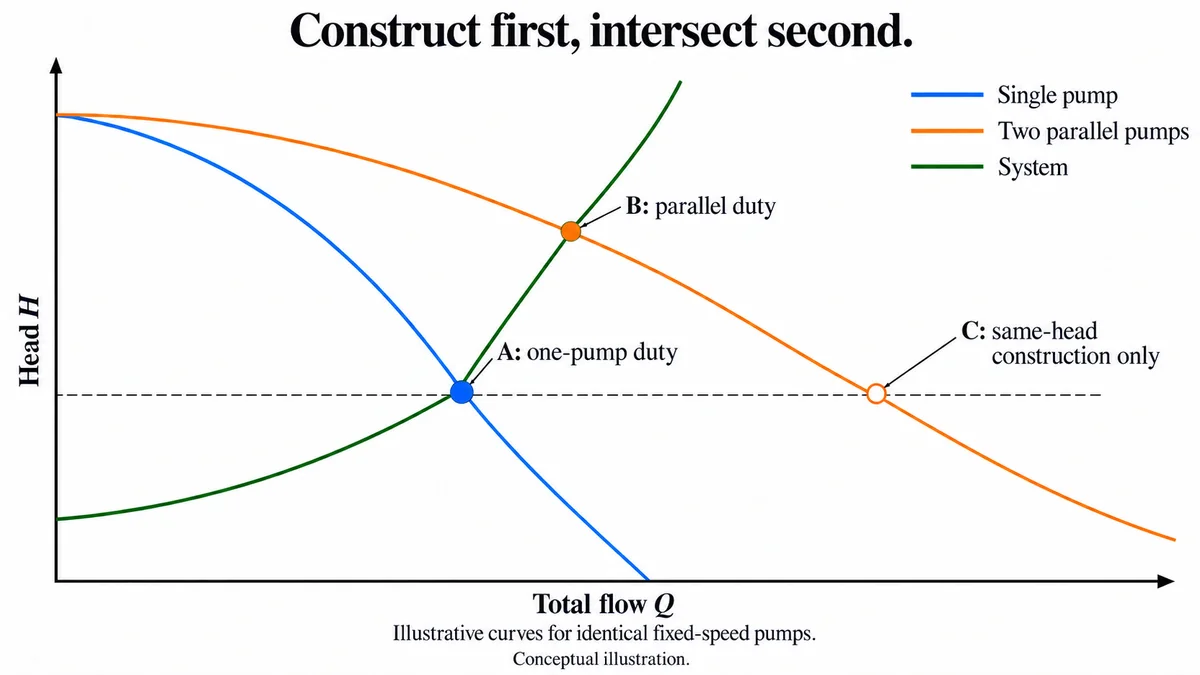
Put total flow on the horizontal axis and head on the vertical axis. For a parallel arrangement with shared suction and discharge boundaries, choose one head, read each pump's flow at that head and add those flows. Repeat at other heads to construct the composite curve. Grundfos explains this horizontal addition; series operation instead adds heads at a common flow. That contrast explains the graph, rather than recommending a change of arrangement.
Now place the system curve on the same axes. It represents the head the system requires at different total flows. Its intersection with the composite curve gives the new operating point. The Hydraulic Institute's parallel-pump explanation shows why a rising system curve normally yields less than twice the previous operating flow.
The order is important: construct first, intersect second. Reading twice the old flow and keeping the old head quietly skips the extra system resistance associated with the increased flow.
A fictional example makes the difference visible
Assume two identical, fixed-speed centrifugal pumps, a stable declining pump curve and unchanged shared system boundaries. The following functions are invented teaching models, with Q in m³/h and H in metres. They are neither product data nor a recommended operating range:
- Single pump: H = 30 − 0.1Q²
- System: H = 10 + 0.1Q²
- Two pumps in parallel, with Q now the total flow: H = 30 − 0.1(Q/2)²
For one pump, equating the first two functions gives Q = 10 and H = 20. At that head each pump could contribute 10, so horizontal addition gives a composite-curve point of total Q = 20, H = 20. But the fictional system would require H = 50 at Q = 20. That constructed point is not a system operating point.
| Point being read | Total flow, m³/h | Head, m | Meaning |
|---|---|---|---|
| One-pump intersection | 10 | 20 | Original fictional duty |
| Parallel construction at the old head | 20 | 20 | On the composite curve only |
| Two-pump intersection | About 12.65 | 26 | New fictional duty |
The two-pump intersection solves 30 − 0.025Q² = 10 + 0.1Q², giving Q² = 160. Each pump contributes about 6.325 m³/h at H = 26. Each therefore delivers less than it did alone, while their combined flow is greater. The example's total increase is about 26.5%, not a prediction for any installed system.
Turn the graph into a useful supplier question
On the actual proposal, mark the single-pump operating point, one common-head addition and the proposed two-pump intersection in different colours. If the supplier's claimed flow is only the addition point, ask for the missing system intersection. If the underlying system has changed, ask which system curve applies to the intended irrigation state rather than comparing unlike duties.
A valid intersection still needs the supplier's checks for suction margin, motor load, minimum flow and the allowed operating region. Unmatched pumps, variable speeds, different fluids or control interactions need their own analysis. Pump count also does not prove duty-standby availability: a capacity graph cannot establish what remains after a failure.
Once delivered flow is established, use it in the wider greenhouse water balance.
Download the curve-reading record
Download the parallel-pump curve-reading CSV. This is a manual worksheet with fixed, explicitly fictional example values and blank proposal fields; it contains no formulas or automatic curve fitting. Open it as UTF-8, comma-separated text, widen and wrap the columns, and save a working spreadsheet copy. Record the common-head addition separately from the system intersection, then identify which point actually supports the offered flow. Do not substitute the example curves for supplier data.